Convolutional Neural Networks Using Shell Scripts

There’s a genre of YouTube videos and blog posts that I often come across on my fyp: “Training a Neural Network From Scratch.” You know the ones. Someone opens a code editor, and proceeds to build a three-layer perceptron while narrating about how they’re doing it “from scratch”. Or the Rust/C++ crowd, who genuinely write lower-level code but still pull in linear algebra crates or at the very least, a properly optimised math library. What if “from scratch” didn’t mean “without libraries”? What if it meant without a real programming language entirely?

So I did what any sane engineer would do. I implemented a full LeNet-5 style convolutional neural network : forward pass, backpropagation, mini-batch SGD, the works; using nothing but Shell scripts and mawk¹ and I have a lot of feelings about it!

Why LeNet-5? Why MNIST? Why Shell Scripts?

LeNet-5 is the granddaddy of convolutional neural networks. Published by Yann LeCun, Léon Bottou, Yoshua Bengio, and Patrick Haffner in their 1998 paper Gradient-Based Learning Applied to Document Recognition ², it was used in production at NCR to read millions of handwritten checks per day. It was,in some sense, the architecture that proved CNNs work. I chose it because it’s small enough to be tractable, complex enough to be interesting, and well-understood enough that I could cross-check my gradients against a PyTorch reference without losing my mind. MNIST because, well, it’s MNIST. It’s the “Hello World” of deep learning. And Shell Scripts? Because I wanted to make a point.

The Architecture at a Glance

Here’s the full network:

Input 28×28×1 (sparse, ~80% zeros skipped)
  └─ Conv1   6 filters 5×5  ──► ReLU ──► MaxPool 2×2  →  12×12×6
  └─ Conv2  16 filters 5×5  ──► ReLU ──► MaxPool 2×2  →  4×4×16 = 256
  └─ FC1    256 → 120        ──► ReLU
  └─ FC2    120 → 84         ──► ReLU
  └─ FC3    84  → 10         ──► Softmax + Cross-entropy

If you’ve seen LeNet-5 before, this is nearly identical to the original, minus batch normalisation, dropout, and momentum (because implementing those using shell scripts would have pushed me over the edge). Plain SGD with learning rate decay. That’s it!

What “No Dependencies” Actually Means

Here’s every tool involved, most of which ship standard with any Linux distro:

Tool	What It Does
`bash`	Orchestrates everything — epoch loops, worker dispatch, argument parsing
`mawk`	All the math — forward pass, backprop, weight init, gradient reduction, SGD updates
`dd` + `od`	Parse the MNIST binary IDX format into human-readable bytes
`shuf`	Shuffle training indices each epoch
`nproc`	Detect available CPU cores for parallelism

Representing a Tensor

This is where things get fun. And by “fun” I mean “the kind of fun that makes you question your life choices at 2 AM.” AWK has no multidimensional arrays. No structs. No typed arrays. What AWK does have is associative arrays: hash tables indexed by strings. That’s it. That’s what you get. So here’s the trick: I flatten everything into 1D integer-keyed arrays and compute the index manually:

# A 24×24×6 convolution output, stored in out1[]
# Index: out1[row * 144 + col * 6 + filter]
out1[or*144 + oc*6 + f] += W1[f*25 + kr*5 + kc] * v

I made use of integer keys because mawk’s hash function for integer keys is faster than for arbitrary strings due to fewer hash collisions, tighter memory access. This single decision gave me a measurable speedup over the naïve syntax that AWK supports.³

We can’t Do Floating-Point Math!?

This is the part that surprised me. Bash has no native floating-point arithmetic. Try this:

echo $(( 3.14 * 2 ))   # syntax error

Yep. Bash scripts can only do integer math. So every single floating-point operation, every multiply-accumulate, every exp(), every log(), every gradient update has to happen inside mawk. When I do need a quick float operation (say, accumulating the running loss), I shell out to AWK inline:

loss_sum=$(awk -v s="$loss_sum" -v l="$loss_val" 'BEGIN{printf "%.6f", s+l}')

It’s ugly but hey it works! But if you were to use other shell languages, like zsh or ksh, you might have access to built-in floating-point support, which could simplify some of the code. But for this project, I stuck with bash and mawk to keep things consistent and to embrace the challenge of working within these constraints.

Sparse Input Trick:

MNIST images are 28×28 = 784 pixels. But here’s the thing: roughly 80% of those pixels are zero (black background). Storing and iterating over 784 values when only ~150 of them matter is wasteful. In Python, you’d barely notice. In AWK, where every array access is a hash lookup, it’s devastating. So during preprocessing, I convert each image into a sparse format:

152 45:128 46:255 47:38 73:192 74:255 ...

The first number is the count of non-zero pixels. Each subsequent entry is pixel_index:raw_value. The forward pass then scatters these sparse inputs across the convolution output:

for(p in sparse) {
    v = sparse[p]; r = int(p/28); c = p%28
    for(kr=0; kr<=4; kr++) {
        or = r - kr; if(or<0 || or>=24) continue
        ...
    }
}

Instead of iterating over all 784 positions and checking if(pixel != 0), I iterate over only the ~150 non-zero entries. That’s roughly a 4.6× reduction in Conv1 multiply-accumulate operations.

Backpropagation:

I’ll be honest, this is the part I’m most proud of, which also took the longest to debug.

The script is 253 lines of dense AWK that implements the complete forward and backward pass for a single training sample. One invocation of the script reads a sparse image, loads all weights from disk, runs the full forward pass, computes cross-entropy loss, and then backpropagates gradients through every single layer. Softmax and cross-entropy loss:

# Numerically stable softmax (subtract max for stability)
max_v = fc3[0]
for(i=1; i<10; i++) if(fc3[i] > max_v) max_v = fc3[i]
for(i=0; i<10; i++) { sm[i] = exp(fc3[i] - max_v); sum_e += sm[i] }
for(i=0; i<10; i++) sm[i] /= sum_e

loss = -log(sm[LABEL] + 1e-10)

The backward pass for softmax + cross-entropy simplifies beautifully to:

\frac{\partial L}{\partial z_i} = \text{softmax}(z_i) - \mathbb{1}[i = y]

Which in AWK becomes:

for(i=0; i<10; i++) d3[i] = sm[i]
d3[LABEL] -= 1

One line for the output gradient. The rest of backprop is just careful chain rule through ReLU (zero out if pre-activation ≤ 0), max pooling (route gradient to the argmax index), and matrix multiplies (transposed weight matrices). It’s the same math as PyTorch. It’s just…in AWK.

A Free Optimisation:

Here’s something delightful I discovered during Conv2. After Conv1 + ReLU + MaxPool, many of the values in pool1[] are zero (thanks to ReLU killing the negatives). So during Conv2’s forward pass, I skip any input that’s already zero:

for(ch=0; ch<6; ch++) for(kr=0; kr<5; kr++) for(kc=0; kc<5; kc++) {
    pi = (or+kr)*72 + (oc+kc)*6 + ch
    if(pool1[pi] == 0) continue    # ← free ~2× speedup
    acc += W2[f*150 + ch*25 + kr*5 + kc] * pool1[pi]
}

This ReLU-induced sparsity cuts Conv2 computation nearly in half. The same trick applies in the fully connected layers. In a normal framework you’d never bother because SIMD vectorisation makes the branch more expensive than the multiply. But in interpreted AWK, skipping a hash lookup and a float multiply is genuinely significant.

Weight Initialisation:

Proper weight initialisation matters. Random uniform weights would cause the network to diverge almost immediately. I use He-Normal initialisation⁴, which sets:

\sigma = \sqrt{\frac{2}{\text{fan\_in}}}

But mawk doesn’t have a Gaussian random number generator. It has rand(), which gives uniform $\mathcal{U}(0,1)$ . So I implemented the Box-Muller transform:

function randn(   u1, u2) {
    do { u1 = rand() } while(u1 <= 0)
    u2 = rand()
    return sqrt(-2*log(u1)) * cos(6.28318530718 * u2)
}
function he(fan_in) {
    return randn() * sqrt(2.0 / fan_in)
}

Poor Man’s Data-Parallel SGD

Training 60,000 images sequentially in AWK would take… let’s just say “longer than my patience”. The key insight is that each training sample’s forward+backward pass is completely independent. So I parallelise across CPU cores using background job control:

for i in "${!BATCH_IDXS[@]}"; do
    mawk -f sample.mawk -v WD="$WD" -v LABEL="$label" "$img" > "$grad_file" &
    
    if (( running >= WORKERS )); then
        wait -n            # wait for ANY one worker to finish
        running=$(( running - 1 ))
    fi
done
wait   # synchronise the batch

Each worker is a separate process that reads the current weights, processes one image, and dumps its gradients to a file. After the batch completes, a reducer averages all the gradient files:

mawk -f reduce_grads.mawk -v BS=16 grad_0.gr grad_1.gr ... grad_15.gr \
| mawk -f update_weights.mawk -v WD="$WD" -v LR=0.01

This is basically data-parallel mini-batch SGD, implemented as Unix pipes. The gradient reducer reads all N gradient files, averages each parameter’s gradient, and pipes the result directly into the weight updater. The pattern sounds simple, but with controlled concurrency it gives near-linear speedups on multi-core machines for this workload.

A dirty little secret!:

Here’s a dirty little secret about this project: every performance-critical file lives in /dev/shm — Linux’s shared memory tmpfs, a RAM-backed filesystem.

/dev/shm/lenet/
├── mnist/train/img_0.sp ... img_59999.sp
├── weights/*.wt
├── grads/grad_0.gr ... grad_15.gr
└── shuffle.txt

Every epoch, multiple workers spawn, each reading ~3,750 image files and writing gradient files. If these lived on an SSD, we’d be I/O bottlenecked immediately. On /dev/shm, reads and writes happen at memory bandwidth. Weights are read from RAM. Gradients are written to RAM. The shuffle list is in RAM. It’s not a GPU. But for a shell script based neural network, it’s the closest thing to “hardware acceleration” I’m going to get.

The Training Loop

Here’s what training actually looks like over ~22,500 steps (~6 epochs):

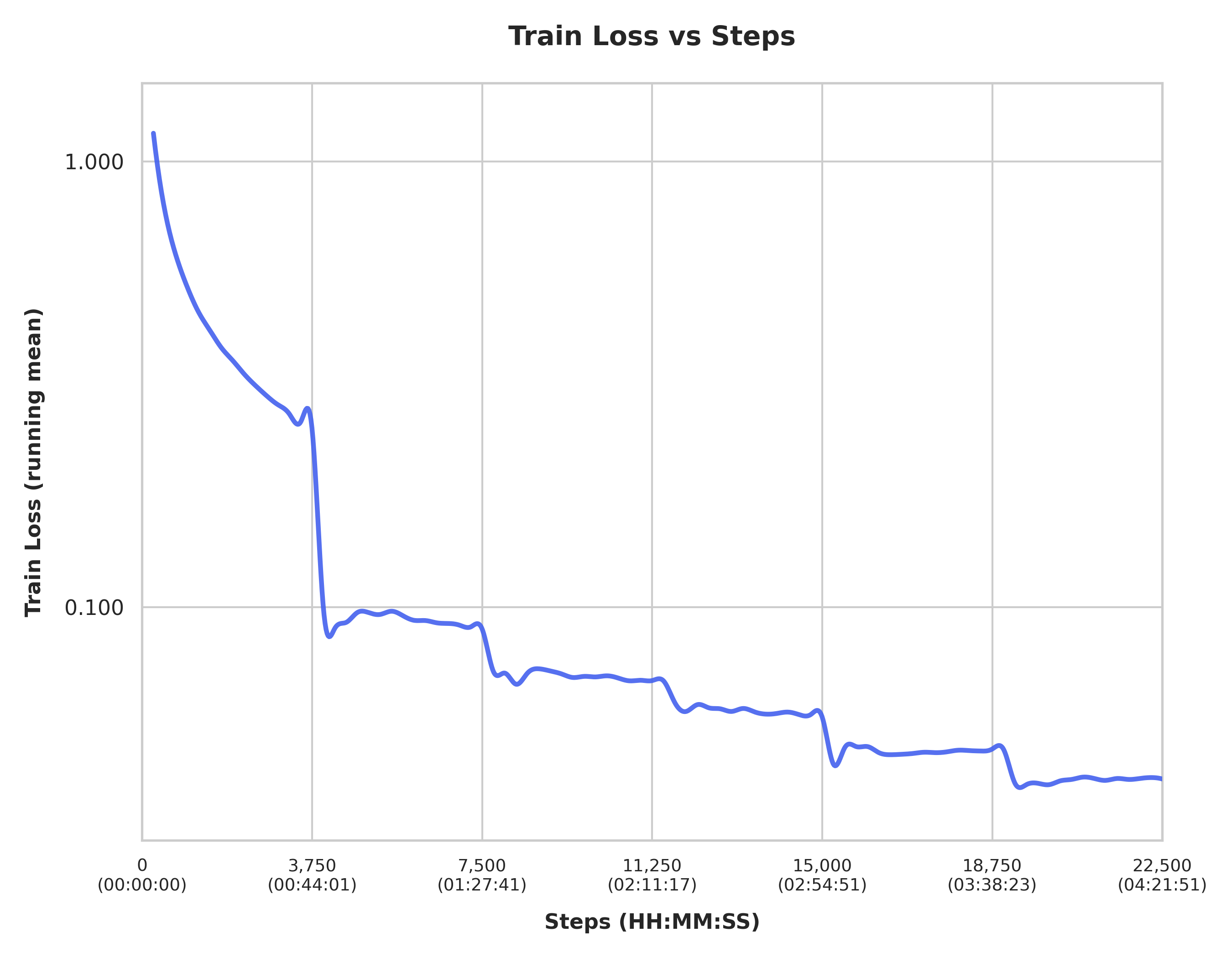
Training loss curve showing smooth convergence from ~1.2 down to ~0.03 over 22,500 steps, with notable step-wise drops at epoch boundaries due to learning rate decay.

It actually converges. The loss starts around 1.2, then drops sharply over the first ~3,750 steps (one epoch), and continues declining smoothly with visible step-wise drops at epoch boundaries from the learning rate decay ( $\text{LR} \times 0.95$ each epoch). By the end of training, we’re sitting at a loss of roughly 0.03. The final test accuracy was 98.47%

What was the Point of doing all this?

I wanted to find out: what is the absolute minimum you need to train a neural network?. The answer, it turns out is:

A way to read and write files
A way to run things in parallel
Patience

You don’t need tensor libraries. You don’t need automatic differentiation. You don’t even need native floating-point support as long as you can call one that does. The math is the math. Convolution is just nested loops and multiply-accumulates. Backpropagation is just the chain rule applied systematically.When you strip away all the abstractions, all the frameworks, all the CUDA, what’s left is exactly what these things actually are: arrays of numbers, being multiplied and added together, over and over, until a loss function gets small.

A Few Honest Limitations:

For starters, it is slower than C/CUDA stacks by a huge margin. For comparison, a PyTorch implementation of this same LeNet-5 trains in about a few seconds on a laptop GPU and hits 99%+ accuracy. So no, it is not going to replace your CUDA kernels. That was never the point. Scaling to larger models would require serious redesign, but for a small demo like this, it’s surprisingly robust. Finally as I have come to realise, maintaining large numeric code in awk is not exactly something sane programmers would like to do.

Try It Yourself

If you’ve got a Linux box with mawk installed (and if you’re on Debian/Ubuntu, you already do), you can run this:

git clone <repo-url>
bash download_mnist.sh   
bash preprocess.sh        
bash init_weights.sh
bash train.sh
bash infer.sh --mode=eval

mawk is Mike Brennan’s fast AWK interpreter — a POSIX text-processing tool that ships with most Linux distros. It is emphatically not a machine learning framework. ↩
Y. Lecun, L. Bottou, Y. Bengio and P. Haffner, “Gradient-based learning applied to document recognition,” in Proceedings of the IEEE, vol. 86, no. 11, pp. 2278-2324, Nov. 1998, doi: https://doi.org/10.1109/5.726791. ↩
Hashing these strings is slower than hashing a single integer, which mawk can internally fast-path. When you’re indexing thousands of weights per forward pass, this adds up. ↩
Kaiming He, Xiangyu Zhang, Shaoqing Ren, and Jian Sun. 2015. Delving Deep into Rectifiers: Surpassing Human-Level Performance on ImageNet Classification. In Proceedings of the 2015 IEEE International Conference on Computer Vision (ICCV) (ICCV ‘15). IEEE Computer Society, USA, 1026–1034. https://doi.org/10.1109/ICCV.2015.123 ↩