How to Train Your GAN

I’ve been trying to make my digital camera produce that gorgeous film look without touching Lightroom. You know, the reasonable approach. So naturally, I decided to train GANs (Generative Adversarial Networks)¹ to achieve this goal and that too on a TPU (Tensor Processing Unit). The thing is, I have never trained a GAN that worked (I had experimented before, but let’s not count those). Also, I’d never touched a TPU. Yes, my strategy for finally succeeding was to add another thing I didn’t understand. Flawless logic.

Why GANs? Why TPUs?

GANs are still one of the most flexible neaural networks that learn a mapping from one image domain to another when you care about perceptual quality. GAN’s are made up of two neural networks : a generator and discriminator where both contest against each other in an adversarial process . A conditional GAN for my use case would consist of a generator that learns to translate input to cinematic output while the discriminator(s) pushes the generator toward photorealistic and style-faithful outputs. For image-to-image translation specifically, GANs learn a loss that adapts to the data, allowing them to learn structured transformations between input and output images.

The TPU choice was pure hubris. Kaggle dangles these TPU accelerators like forbidden fruit², and I bit. Hard. TPUs are application-specific integrated circuits (ASICs) designed by Google for neural network machine learning, optimized for high volumes of low-precision computation with specialized matrix multiply units. Translation: they’re really, really good at the kind of math that neural networks love. Plus, admit it: telling someone you trained on a TPU just sounds cooler. I’m only human. If you want to know more about TPUs, Google has got a great blog explaining everything that you can access here. But, as I quickly learned, with great power comes great frustration. TPUs are strict. When something breaks on a TPU, it breaks spectacularly.

Model Architecture

To train a GAN you either can utilize either paired images (an image in one domain and its corresponding look in the target domain) or unpaired images (just random images from source and target domains). I managed to find a dataset which had paired images: the normal input and the same scene with cinematic filters applied. I did some digging and found out about Pix2Pix.³. Inspired by the paper I tried to create my own implementation.

Generator:

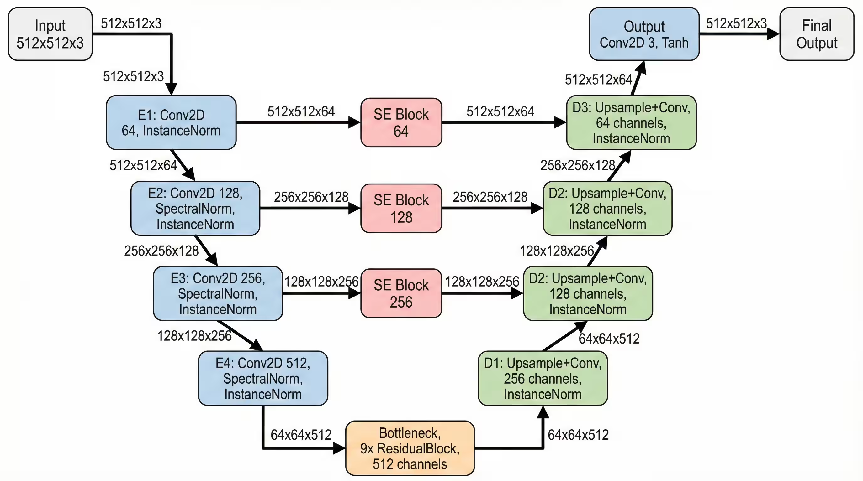
I went with a modified Res-U-Net. It combines the skip-connections of a U-Net⁴ (which preserve structural details like edges by passing them directly from the encoder to the decoder) with the depth of Residual Blocks (which prevent the vanishing gradient problem in deep networks).

But I made some specific “chef’s choice” architectural decisions to avoid common GAN pitfalls:

• Instance Normalisation: Instance normalisation is independent of batch size and does not introduce correlations across a batch, which can prevent the “leakage” of information between samples that sometimes causes artifacts in GANs ⁵

• Pixel Shuffle (Depth-to-Space): If you’ve ever seen a GAN-generated image that looks like it has a faint checkerboard grid overlaid on it, that’s the fault of the Standard Transposed Convolution (Deconv) layer. It’s a result of uneven overlap during the upsampling process. I used a technique known as “Pixel Shuffle.”⁶ It generates four times the channels in the lower resolution and then rearranges them mathematically into a larger spatial resolution. It’s cleaner, sharper, and completely eliminates the checkerboard artifact.

• Squeeze & Excitation Blocks⁷: Each upsample got its own S-E Block from the skip connection, because the model should choose which details to remember, not just blindly concatenate everything like a hoarder.

Also I used like nine residual blocks. Nine! I figured if ResNet could go 50 layers deep for ImageNet, I could damn well spend some compute on aesthetics.

Discriminator:

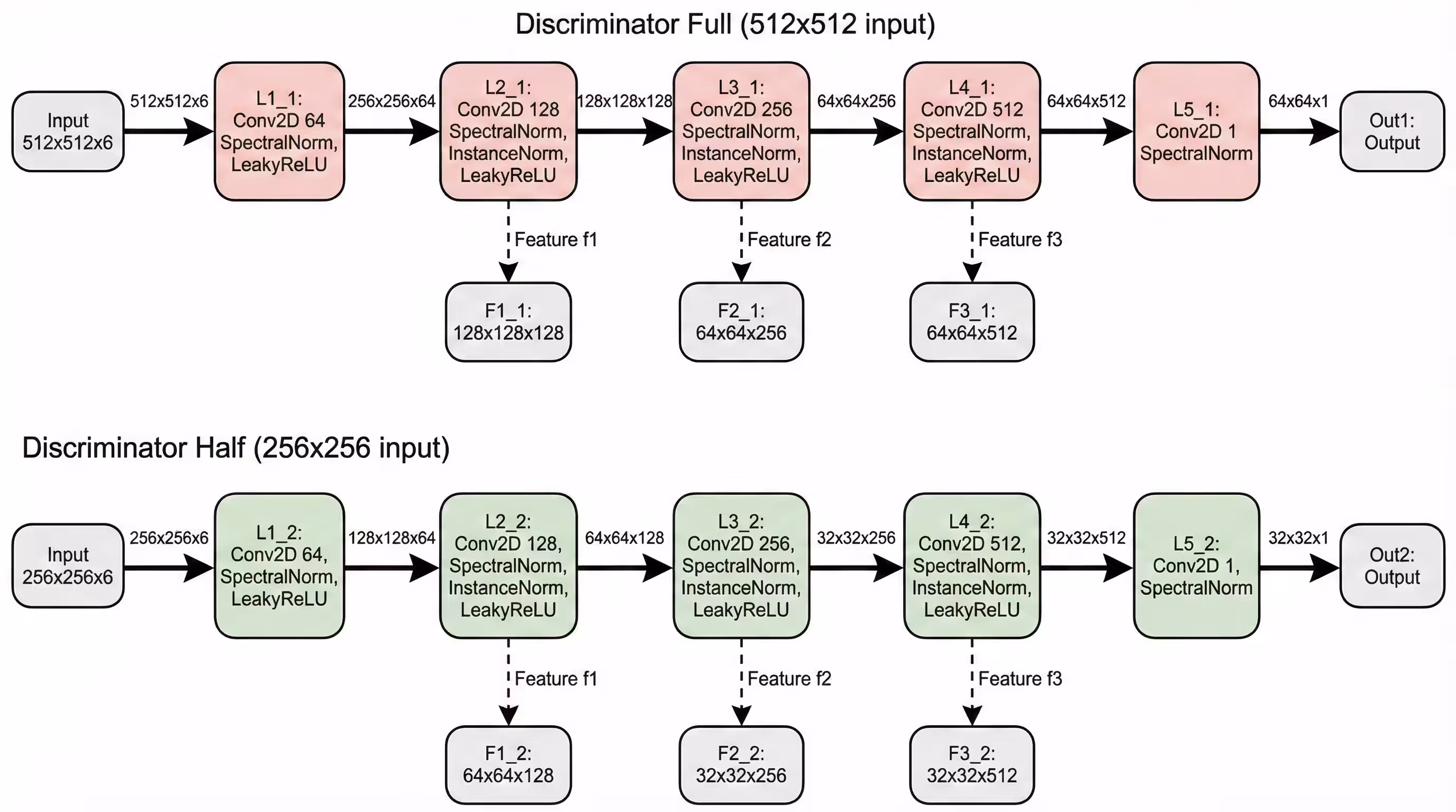
I went with a Multi-Scale Spectral PatchGAN⁸, because for me one discriminator wasn’t enough.

• Discriminator 1 looks at the full 512x512 image. It critiques the composition and global lighting.
• Discriminator 2 looks at a downsampled 256x256 version. It critiques the broader structure. This ensures the model gets the global structure right while also nailing the local textures. I also wrapped everything in Spectral Normalization. This is a fancy term for a mathematical leash. It constrains the Lipschitz constant of the network, which basically prevents the Discriminator from becoming too smart too fast.

Why use such a complex architecture you ask? Because why use one trendy architecture when you can weld three together with prayers.

Loss Functions

Training GANs is an art of balancing multiple objectives. Here’s what I threw into the mix:

1. Adversarial Loss :

For the discriminator:

def discriminator_loss(real_output, fake_output):
    real_output = tf.cast(real_output, tf.float32)
    fake_output = tf.cast(fake_output, tf.float32)
    real_loss = tf.reduce_mean(tf.maximum(0.0, 1.0 - real_output))
    fake_loss = tf.reduce_mean(tf.maximum(0.0, 1.0 + fake_output))
    return real_loss + fake_loss

This hinge loss formulation encourages the discriminator to be confident (outputs > 1) about real images and confident (outputs < -1) about fake ones, with a margin for error.

For the generator:

def generator_loss(fake_output):
    fake_output = tf.cast(fake_output, tf.float32)
    return -tf.reduce_mean(fake_output)

The generator simply tries to maximize the discriminator’s output on fake images.

2. Feature Matching Loss

Instead of just caring about the final discriminator output, I also matched intermediate feature representations:

def feature_matching_loss(real_features, fake_features):
    loss = 0
    for real_f, fake_f in zip(real_features, fake_features):
        real_f = tf.cast(real_f, tf.float32)
        fake_f = tf.cast(fake_f, tf.float32)
        loss += tf.reduce_mean(tf.abs(real_f - fake_f))
    return loss

This uses the [f1, f2, f3] feature outputs from the discriminator, computing L1 distance at each level:

$$\mathcal{L}_{FM} = \sum_{i=1}^{3} \mathbb{E}[||D_i(x, y) - D_i(x, G(x))||_1]$$

Feature matching stabilizes training by giving the generator more detailed feedback about what’s wrong with its outputs.

3. Perceptual Loss (VGG Features)

The most computationally expensive but arguably most important loss. I used a pre-trained VGG19⁹ to extract features from the ‘block4_conv2’ layer. The key optimisation that I did here was batching real and target images together for a single VGG forward pass instead of two separate ones. This nearly doubled training speed.

Total Loss

The final generator loss combines all three:

$$\mathcal{L}_{G} = \lambda_{GAN} \mathcal{L}_{GAN} + \lambda_{FM} \mathcal{L}_{FM} + \lambda_{VGG}\mathcal{L}_{VGG}$$

With weights: $\lambda_{GAN}=1.0, \lambda_{FM} = 10.0, \lambda_{VGG} = 2.0$

Optimizing for TPU’s

I could have just written code good enough to just make it run, but my previous experiences with GPUs have taught me to optimize as much as possible otherwise you could be waiting for a long time for your model to train. So I looked up a few things on how to optimize code on TPU’s and here are a few things that worked for me :

1. Mixed Precision Training:

The first and most crucial optimisation:

with strategy.scope():
    policy_type = 'mixed_bfloat16' if isinstance(strategy, tf.distribute.TPUStrategy) else 'mixed_float16'
    mixed_precision.set_global_policy(policy_type)
    print(f"Mixed Precision Policy: {policy_type}")

TPUs love bfloat16¹⁰. The hardware is literally built for it. This reduces memory usage and increases throughput significantly. However, loss calculations must stay in float32 to maintain numerical stability

2. Data Pipeline Optimisation

The TPU can compute faster than most storage systems can feed it data. The solution:

train_dataset = train_dataset.map(load_paired_images, num_parallel_calls=AUTOTUNE)
train_dataset = train_dataset.cache()  # Cache decoded images in RAM
train_dataset = train_dataset.map(augment, num_parallel_calls=AUTOTUNE)
train_dataset = train_dataset.batch(BATCH_SIZE, drop_remainder=True)
train_dataset = train_dataset.prefetch(AUTOTUNE)

The .cache() call is crucial because it stores decoded images in memory after the first epoch, eliminating repeated decoding overhead. Combined with prefetch(AUTOTUNE), this kept the TPU fed with data.

3. Batch Resizing

Instead of resizing images twice (once for each discriminator), I did this:

# Batch resize all images at once
combined_images = tf.concat([input_image, target_image, fake_image], axis=0)
combined_half = tf.image.resize(combined_images, [IMG_SIZE // 2, IMG_SIZE // 2])
input_half, target_half, fake_half = tf.split(combined_half, 3, axis=0)

Three resizes become one. Small optimization, but every millisecond counts when you’re running lots of training steps.

4. Distributed Training Setup

Each TPU core processes a mini-batch independently, then all losses are summed and averaged. The @tf.function decorator compiles this into a XLA graph that runs natively on the TPU.

@tf.function
def distributed_train_step(input_image, target_image):
    def train_step_wrapper(input_img, target_img):
        return train_step(input_img, target_img, generator, discriminator1, 
                         discriminator2, vgg_model, gen_optimizer, disc_optimizer)
    per_replica_losses = strategy.run(train_step_wrapper, args=(input_image, target_image))
    
    # Reduce and average losses across replicas
    num_replicas = tf.cast(strategy.num_replicas_in_sync, tf.float32)
    total_gen_loss = strategy.reduce(tf.distribute.ReduceOp.SUM, per_replica_losses[0], axis=None) / num_replicas
    # ... (reduce other losses similarly)
    
    return total_gen_loss, total_disc_loss, gen_gan_loss, gen_fm_loss, gen_vgg_loss

Removing Artifacts

After training the model for 50 epochs. The results were… interesting. The colors were kinda cinematic, but there were strange artifacts. The lights were “blooming” too aggressively.

The Fix: Total Variation Loss

I decided to fine-tune for another 20 epochs, but I needed to punish the model for being noisy. Enter Total Variation Loss. TV Loss is a concept borrowed from classic image processing (before AI took over). It measures the difference between adjacent pixels. If a pixel is vastly different from its neighbor (which looks like noise), the loss goes up. It forces smoothness where edges aren’t explicitly required. I added this to the training loop with a heavy weight and lowered the learning rate. The new loss looked like :

$$\mathcal{L}_{G}^{finetune} = \mathcal{L}_{GAN} + 10\mathcal{L}_{FM} + \mathcal{L}_{VGG} + 20\mathcal{L}_{TV}$$

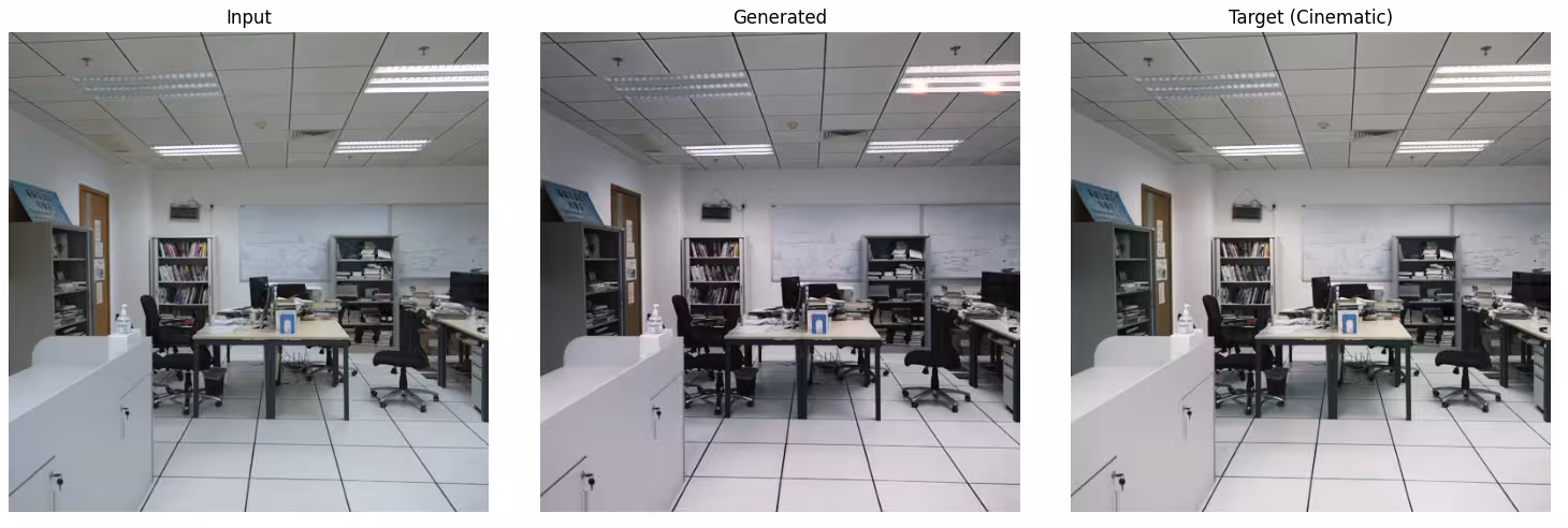
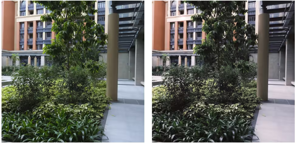
Results

Worth the headache?

Absolutely. Training on TPUs turned what would’ve been a week-long project into a weekend adventure. Along the way I had to deal with so many errors that sometimes I was on the brink of tearing my hair out! The final model isn’t perfect. It still generates weird artifacts or misses the mark on certain image types. But it successfully learned to apply a consistent cinematic aesthetic to arbitrary photographs, which was the goal. And I got to play with some seriously powerful hardware in the process. I could have probably saved myself 20 epochs of pain by reading more papers first. But where’s the fun in that?

If you want to dive deeper into the code, check out the full training notebook here.

Now if you’ll excuse me, I have some more “experiments” to run. I wonder what happens if I increase the resolution to 1024×1024…

Footnotes

1. https://arxiv.org/abs/1406.2661 ↩

2. https://www.kaggle.com/docs/tpu ↩

3. https://arxiv.org/abs/1611.07004 ↩

4. https://arxiv.org/abs/1505.04597 ↩

5. https://www.rohan-paul.com/p/ml-interview-q-serieshow-do-batch ↩

6. https://arxiv.org/abs/1609.05158 ↩

7. https://arxiv.org/abs/1709.01507 ↩

8. https://arxiv.org/abs/1711.11585 ↩

9. https://arxiv.org/abs/1409.1556 ↩

10. https://cloud.google.com/blog/products/ai-machine-learning/bfloat16-the-secret-to-high-performance-on-cloud-tpus ↩